Simple Facts About \(\:\chi^2\) Distribution Shapes

June 28, 2024

A Visual Motivation

When we first learn about probability distributions, we might first see the beauty of normal (Gaussian) distributions, understand its density function and bell-shaped curve, then study many related distribution.

One of the interesting distribution is the chi-squared \(\chi^2\) one. Given \(k\) i.i.d. standard normal variables \(X_1, ..., X_k\), if we denote \begin{equation} Z_k = X_1^2 + \cdots + X_k^2 = \sum_{i=1}^k X_i^2 \tag{1} \end{equation} then \(Z_k \sim \chi^2_k\), a chi-squared R.V. with \(k\) degrees of freedom. \(Z_k\) has density \begin{equation} f_{Z_k}(z) = \frac{1}{2^{k/2}\Gamma(k/2)} z^{k/2 - 1} e^{-z/2} \tag{2} \end{equation} and its expectation and variance are \(k\) and \(2k\) respectively. ⊕
Figure 1: Chi-squared distributions with different degrees of freedom.
In the lecture, we might have seen the following graph for chi-squared distributions with different degrees of freedom \(k\) (see RHS).

My immediate response when seeing this picture was: what makes the difference between \(k \leq 2\) and \(k > 2\)? For the cases where \(k = 1 \:\text{or}\: 2\), we observe

1. The density at \(x = 0\) is non-zero, while later on they all become zero.
2. The density also reaches its mode at \(0\) on the x-axis, while later on they all peak at \(x > 0\).
3. The density function overall is convex and monotonic decreasing, but when \(k > 2\), convexity/concavity changes.

Most important, as we should remember that \(\chi^2\) is a special case of the more general gamma distribution, we want to make sure whether \(k = 2\) (an integer degree of freedom) is the real boundary between the two “shape behaviors”, or whether we can find a more precise boundary by allowing \(k\) to take arbitrary values in \(\mathbb{R}^+\).

Level I: \(\:\chi^2\) At the Origin

As a warm-up exercise, we investigate the density function at the origin. From here on, we will resume using \(f_{Z_k}(z)\) as the p.d.f. At \(z = 0\), we have \begin{equation} f_{Z_k}(0) = \frac{1}{2^{k/2}\Gamma(k/2)} \cdot 0^{k/2 - 1} e^{-0/2} \tag{3} \end{equation} For any \(k \in \mathbb{R}\) such that \(k > 2\), since \(0^{k/2 - 1} = 0\), we have \(f_{Z_k}(0) = 0\) without any issue. This explains the above graph where the density at \(0\) is zero for \(k > 2\). As a direct result, the p.d.f for chi-squared distribution cannot be always convex or monotonically decreasing after this threshold.

Next, when \(k = 2\) exactly, we are faced with the indeterminate form \(0^0\) in the expression. A simple solution is to consider the limit of the density function as \(z \to 0\): \begin{equation} \lim_{z \to 0} f_{Z_2}(z) = \lim_{z \to 0} \frac{1}{2\Gamma(1)} z^0 e^{-z/2} = \frac{1}{2} \tag{4} \end{equation} as \(\Gamma(1) = 1\). We can happily use this as a “definition” for the density at origin to ensure continuity. Finally, as \(k < 2\) (i.e. \(k/2 - 1 < 0\)), we have: \begin{equation} \lim_{z \to 0} z^{k/2 - 1} = \infty \tag{5} \end{equation} thus making the p.d.f diverge at the origin.

Level II: Diving Into the Maximizer

⊕
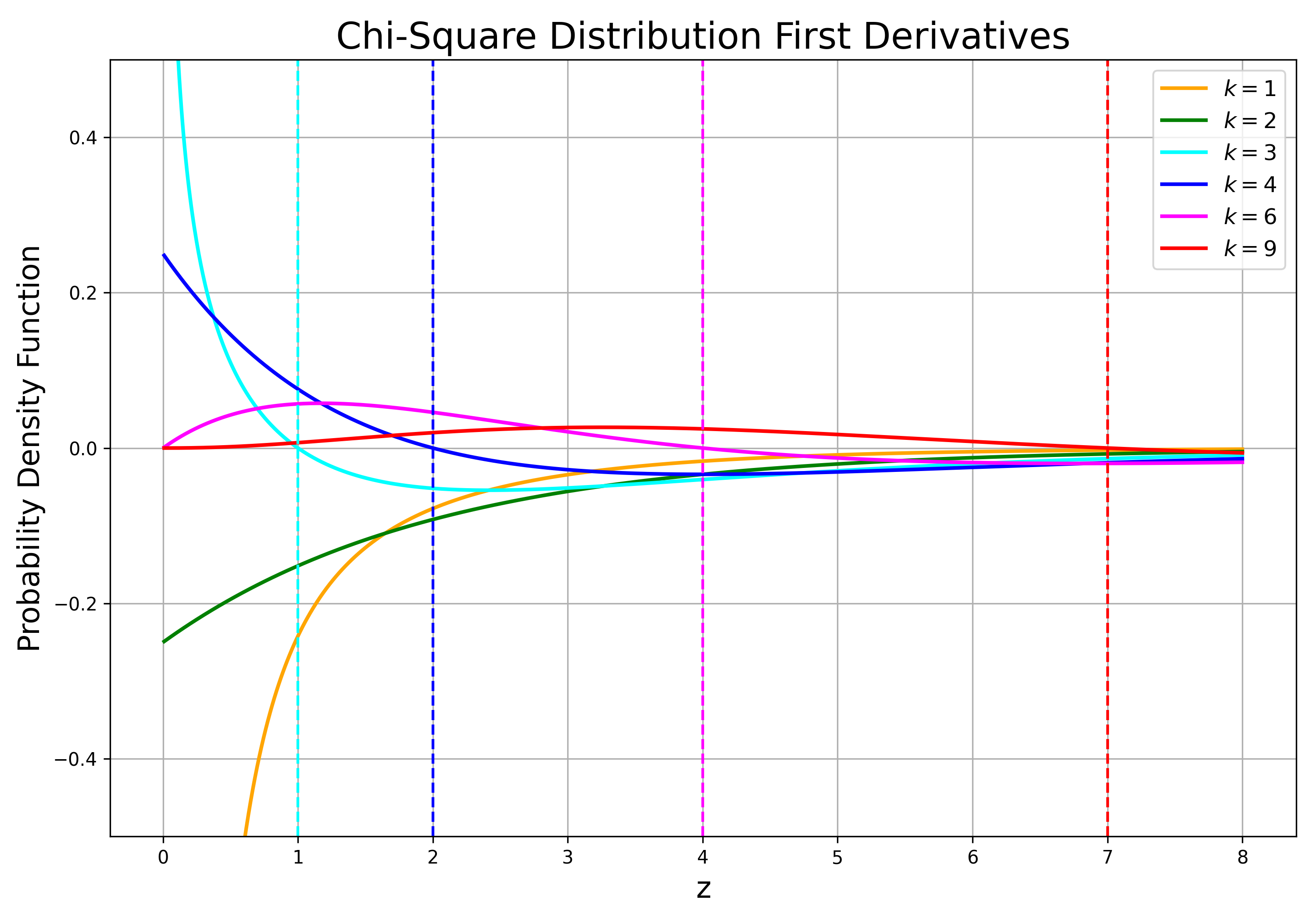
Figure 2: First derivatives for Chi-squared p.d.f(s)
Now we turn to the mode of the chi-squared distribution. This question is quite dumb when \(k < 2\), as we just found out that the density function diverges at the origin. In general, we take the derivative and have: \[\begin{align} \frac{d}{dz} f_{Z_k}(z) &= \frac{1}{2^{k/2}\Gamma(k/2)} \left[ (k/2 - 1) z^{k/2 - 2} e^{-z/2} - \frac{1}{2}z^{k/2 - 1} e^{-z/2} \right] \newline &= \frac{1}{2^{k/2}\Gamma(k/2)} z^{k/2 - 1} e^{-z/2} \left[\frac{k}{2z} - \frac{1}{z} - \frac{1}{2}\right] \newline &= \left[ \frac{k - z - 2}{2z} \right] f_{Z_k}(z) \tag{6} \end{align}\] when \(k = 2\), the derivative equals to \(-2\cdot f_{Z_2}(z)\), which is zero only when \(f_{Z_2}(z) = 0\) — something only happens when we take \(z \to \infty\).

When \(k > 2\), we can explicitly solve for \begin{equation} \frac{d}{dz} f_{Z_k}(z) = 0 \iff z = k - 2 \tag{7} \end{equation} where each p.d.f reaches the peak at \(z = k - 2\).

Level III: The Myth of Convexity

Finally, we want to numerically verify the convexity/concavity of the chi-squared density function through the lens of the second derivative. By recursion, we have \[\begin{align} \frac{d^2}{dz^2} f_{Z_k}(z) &= \left[ \frac{k - z - 2}{2z} \right] \frac{d}{dz} f_{Z_k}(z) + \left[ \frac{2-k}{2z^2} \right] f_{Z_k}(z) \newline &= \left[ \frac{(k - z - 2)^2 + 4 - 2k}{4z^2} \right] f_{Z_k}(z) \end{align}\] Once again, since the density itself is nonnegative, we only need to focus on the first term. For \(k < 2\), we have \(4 - 2k > 0\), so the first term is always positive. Thus we have a positive second derivative (“curvature”) for all \(z\) and the density is convex. Similar things happen when \(k = 2\), as the second derivative is always positive as long as \(z > 0\).

When \(k > 2\), convexity/concavity changes over different combinations of \(z\) and \(k\). As we can see from Figure 2, the density might turn from being concave to convex, or the other way around.